Accurate monitoring of Above-Ground Biomass (AGB) is essential to quantify planetary carbon stocks and understand the impacts of forest degradation on terrestrial biodiversity. While spaceborne LiDAR, particularly from the NASA GEDI mission, has revolutionized AGB estimation by providing high-resolution vertical profiles of vegetation, these observations remain spatially sparse. Conversely, existing wall-to-wall global biomass products typically rely on lower resolution data, which often fail to capture fine-grained forest structures and introduce biases when upsampled. In this study, we propose a unified approach to generate high-resolution (10 m) dense AGB maps across diverse geographical regions. We introduce BioFiLM, an architecture that utilizes frugal Feature-wise Linear Modulation (FiLM) layers to adapt a shared base model to different vegetation types, outperforming both biome-agnostic models and biome-specific ensembles in terms of accuracy and efficiency. To address the spatially structured residuals and biases typical of large-scale AGB products, we develop a post-hoc calibration scheme using Gaussian Process Regression (GPR). By leveraging the spatial covariance of prediction errors, the GPR framework allows for localized corrections of AGB estimates. Our results show that this spatial error modeling significantly reduces the observed biases. The robustness of the calibration is validated on an independent site in Sumatra and applied to the ESA CCI biomass product, demonstrating its broad applicability. We provide a dense AGB map covering 3 million km² across 11 globally distributed regions, made accessible via Google Earth Engine to support regional carbon accounting and conservation monitoring.
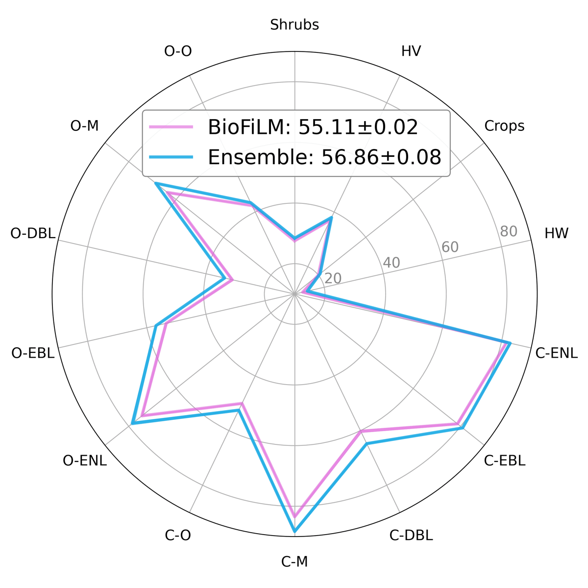
FiLM layers conditioned on biome and region lower the test RMSE on AGBD to 55.11 Mg/ha (baseline: 56.68), and beat an ensemble of 14 biome-specific models (56.86) with 14× fewer parameters.
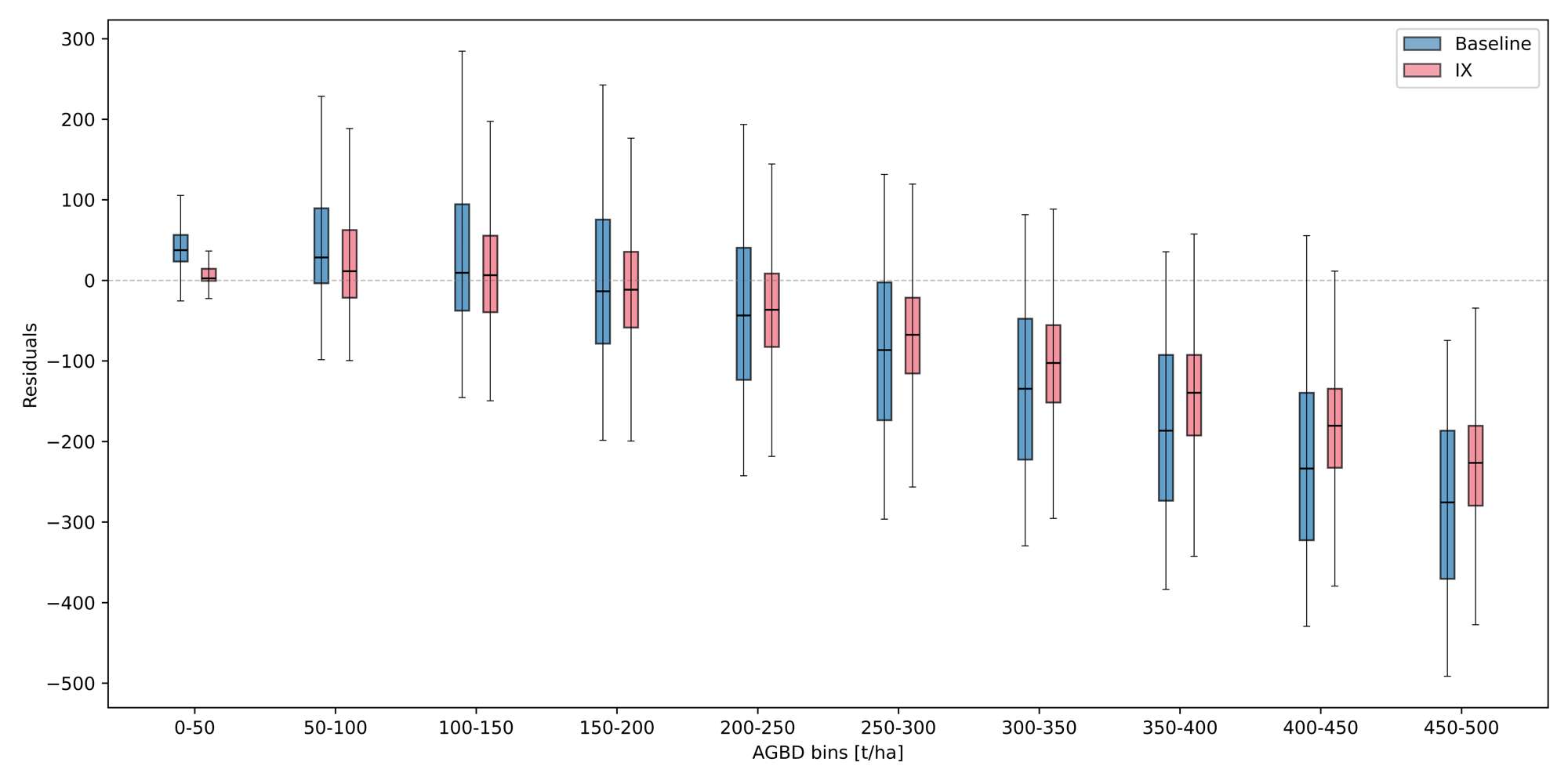
Per-tile kriging of the residuals at GEDI footprints reduces RMSE by 28% and MAE by 45%, shrinks the mean error from 32.61 to 6.11 Mg/ha, and reduces the median bias in all ten 50 Mg/ha bins.
In Jambi (Sumatra), outside the training regions, our map has an RMSE of 38.31 Mg/ha against independent field/ALS reference data, versus 67.58 for ESA CCI.
Applied to the ESA CCI biomass map, the same calibration lowers its RMSE from 67.58 to 47.24 Mg/ha (−30%). Our calibrated 10 m maps cover 3M km² in 11 regions.
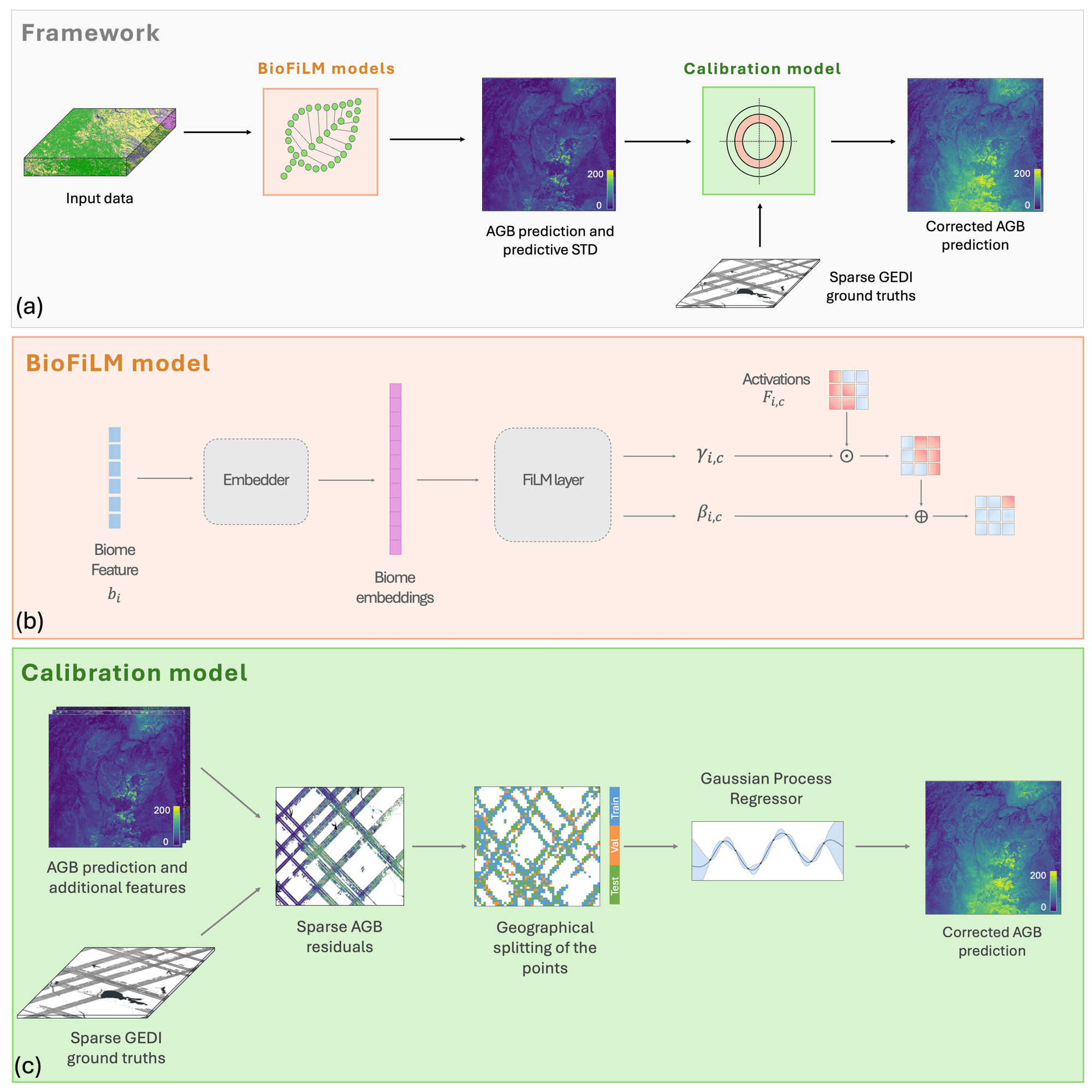
The same tree size or photosynthetic activity can correspond to different biomass in different biomes, because of differences in wood density and allometry. Rather than training one model per biome, BioFiLM adapts a single fully convolutional, Xception-style network (1M parameters, trained with sparse GEDI L4A supervision) with Feature-wise Linear Modulation. The biome (Copernicus land cover) and region are embedded by a small network, and FiLM layers predict a per-channel scale and shift for the activations $F_{i,c}$: $$\mathrm{FiLM}(F_{i,c} \mid \gamma_{i,c}, \beta_{i,c}) = \gamma_{i,c}\, F_{i,c} + \beta_{i,c}.$$ Inputs are Sentinel-2 L2A, ALOS PALSAR-2, the ALOS DSM, land cover and canopy height from the AGBD dataset, plus added topographic (slope, aspect) and temporal (acquisition date, day of year) features.
Like other models of long-tailed vegetation variables, the network over-estimates low biomass and under-estimates high biomass, and the errors are spatially structured. For every Sentinel-2 tile (100×100 km), we:
The GP inputs are the pixel position, the predicted AGB and its ensemble STD (base), neighbourhood statistics (local mean, standard deviation, coefficient of variation and range; local), and Sobel and Laplacian edges (texture). Footprints are split into train / validation / test sets by geographically separated patches, the $x$/$y$ length-scales are set per tile from the footprint spacing, and low-biomass outliers are removed before fitting.
| Model | biome | topo | temporal | FiLM | RMSE (↓) |
|---|---|---|---|---|---|
| baseline | sine-cos | × | × | × | 56.68 Β± 0.03 |
| baseline+ | cat2vec | ✓ | ✓ | × | 55.31 Β± 0.01 |
| BioFiLM | cat2vec | ✓ | ✓ | ✓ | 55.11 Β± 0.02 |
Table 1. Test RMSE (Mg/ha, ↓) on the hold-out AGBD test set, mean Β± std over three runs. baseline+ adds the best combination of extra features to the AGBD baseline; BioFiLM further adds FiLM layers. Best in bold, second best underlined.
Topographic features help consistently; temporal features help only together with them. The best BioFiLM configuration uses a 64-dimensional MLP embedding of one-hot biome and region, FiLM layers in the entry block only, a long-skip connection and light L2 regularization. Placing FiLM in the entry block and adding the region consistently beat all-layer placement and biome-only conditioning.
Figure 1. Overall and per-biome test RMSE (Mg/ha) of BioFiLM (pink) and an ensemble of biome-specific models (blue), one per Copernicus vegetation type. BioFiLM has the lower error in most biomes, and overall, with a single shared model.
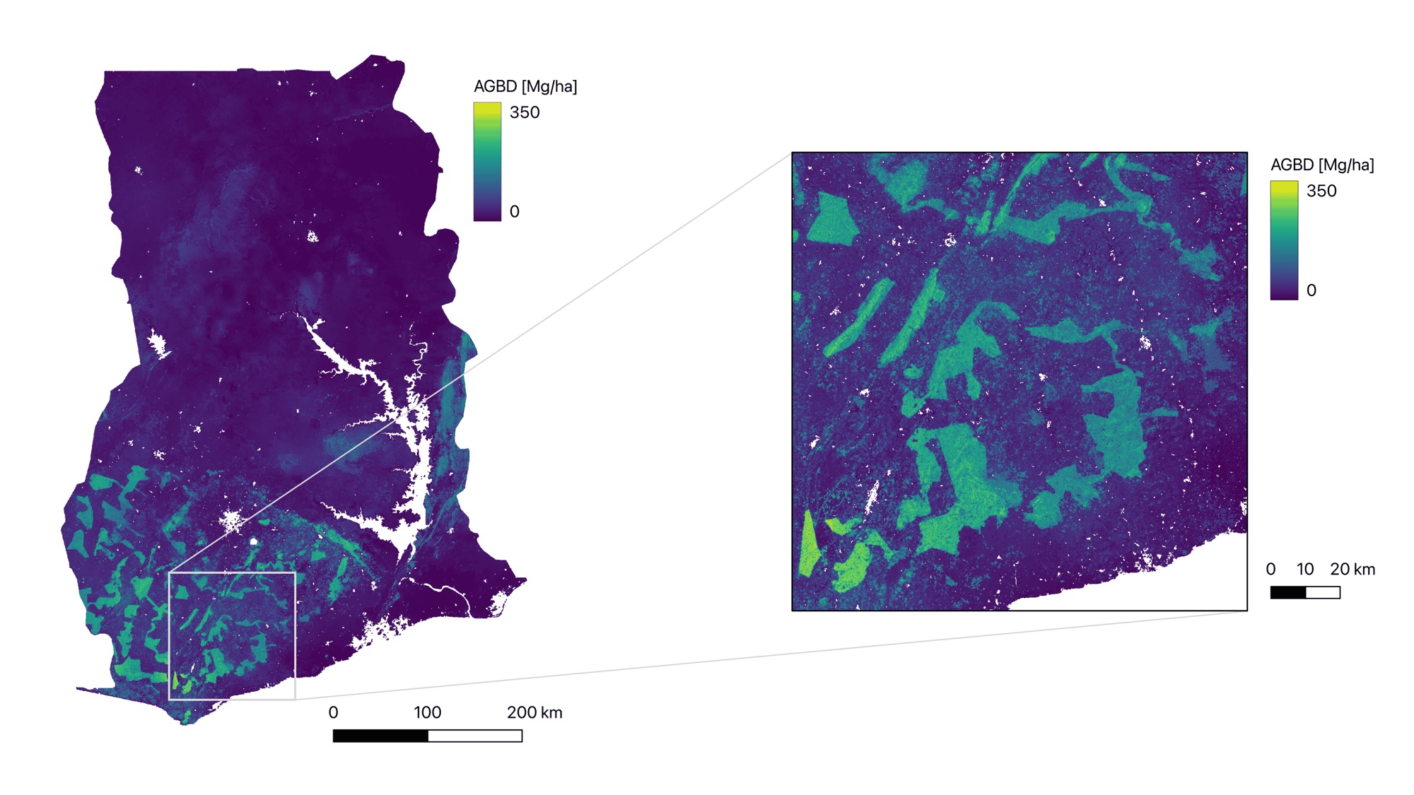
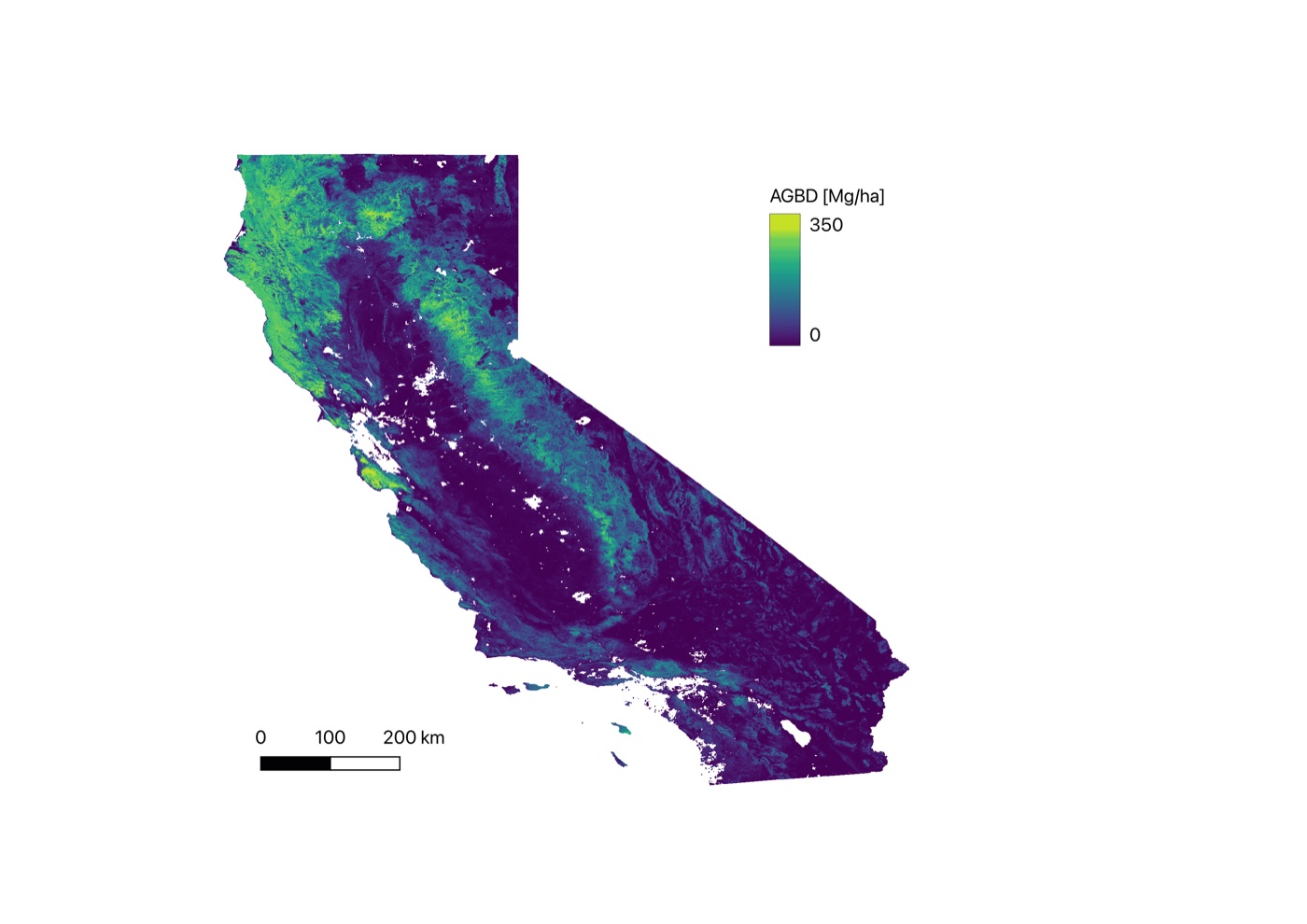
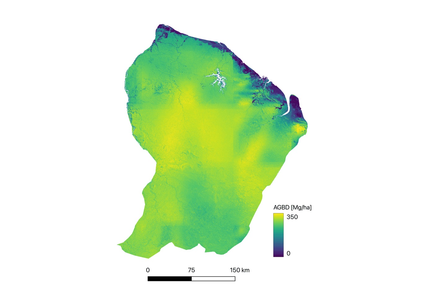
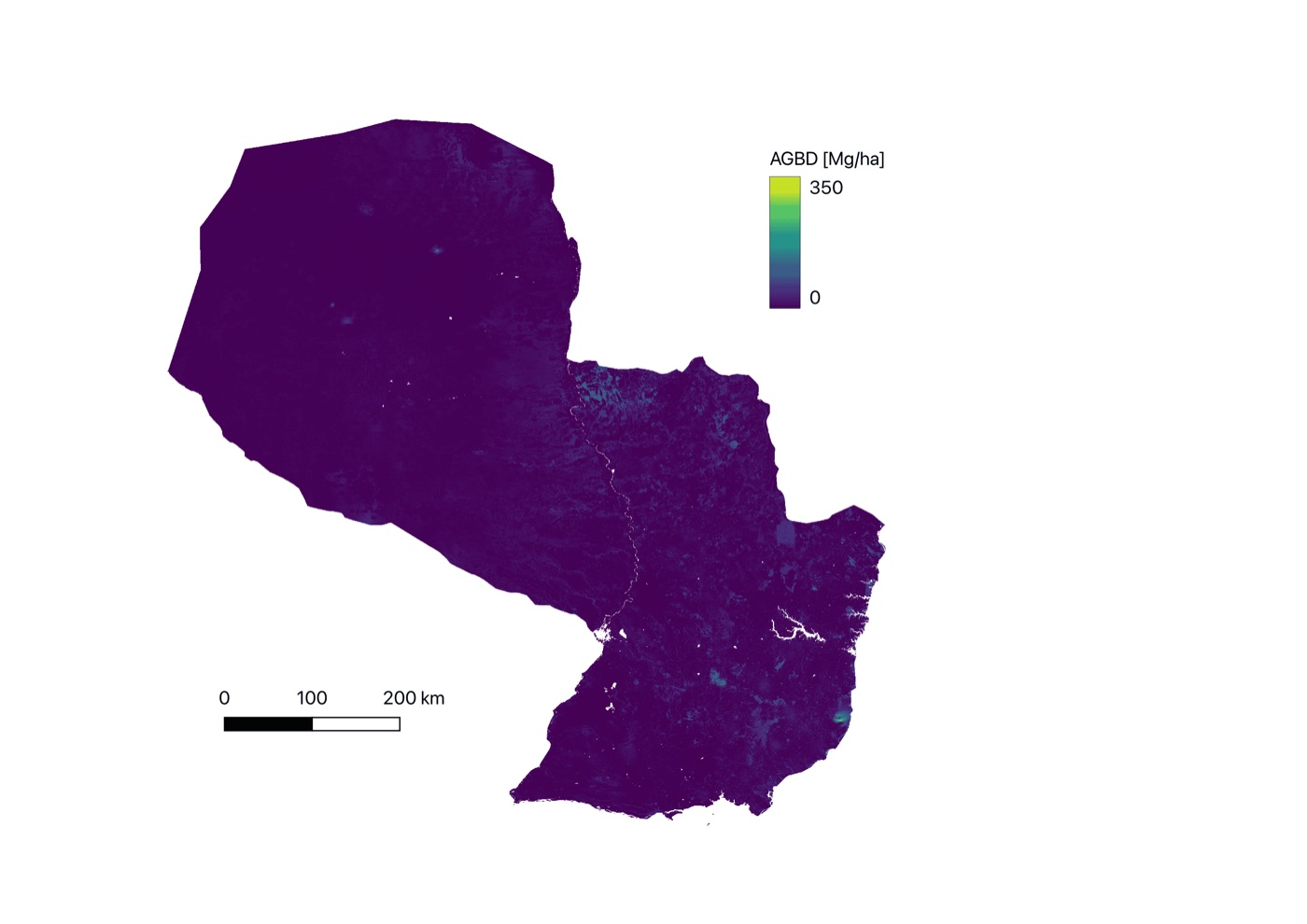
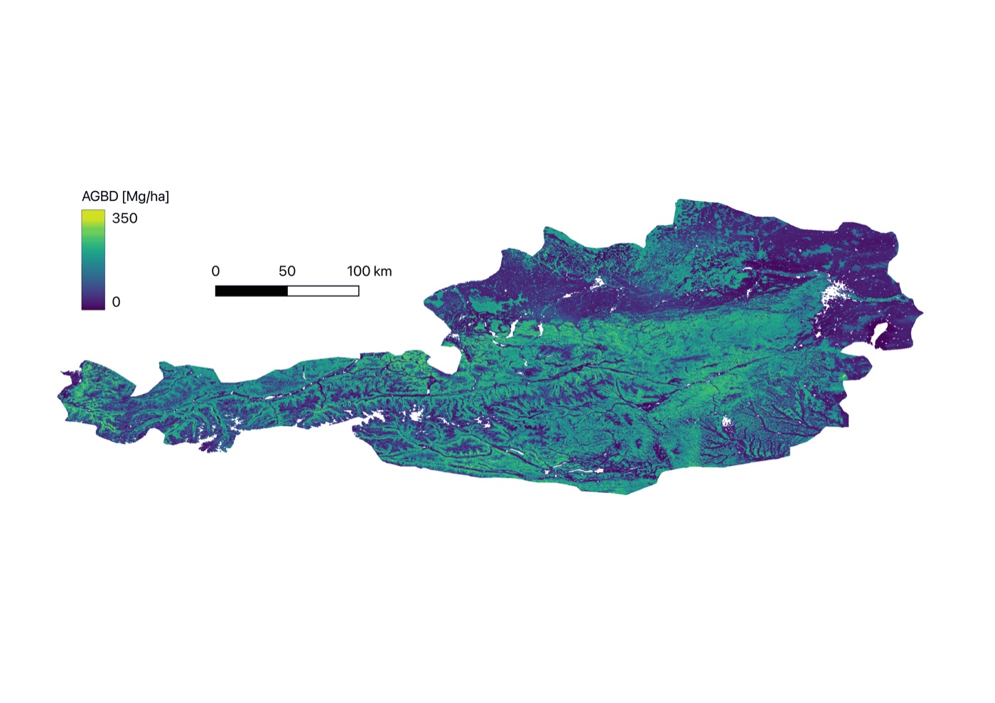
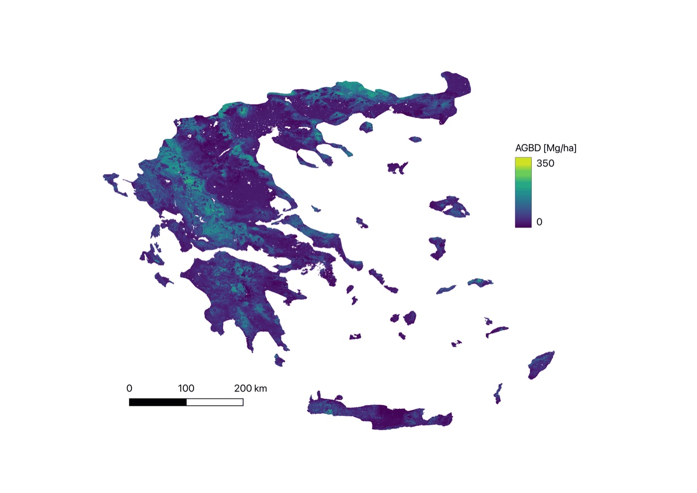
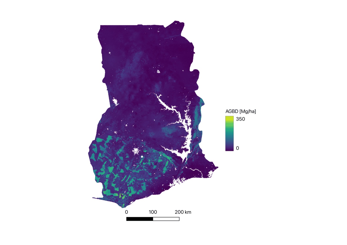
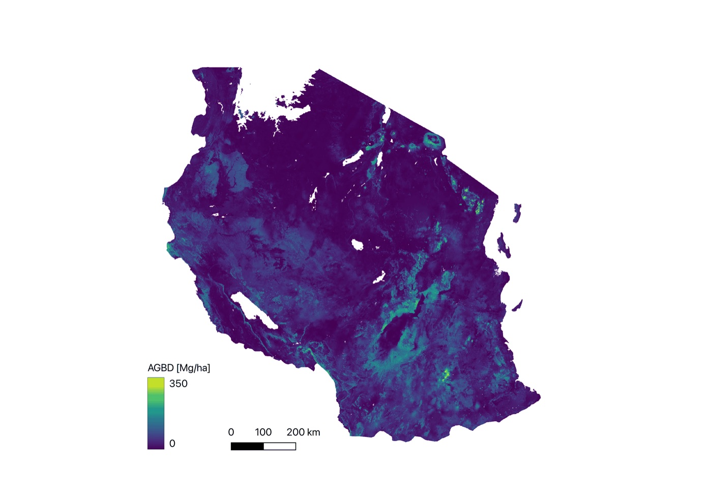
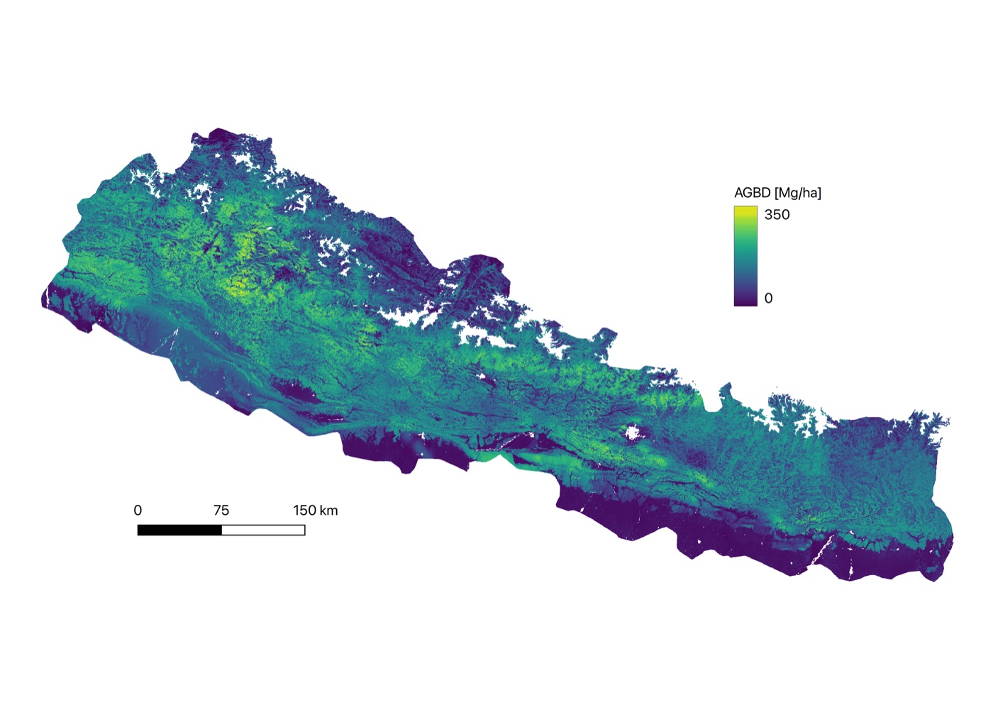
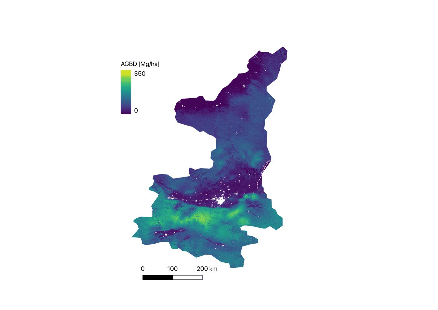
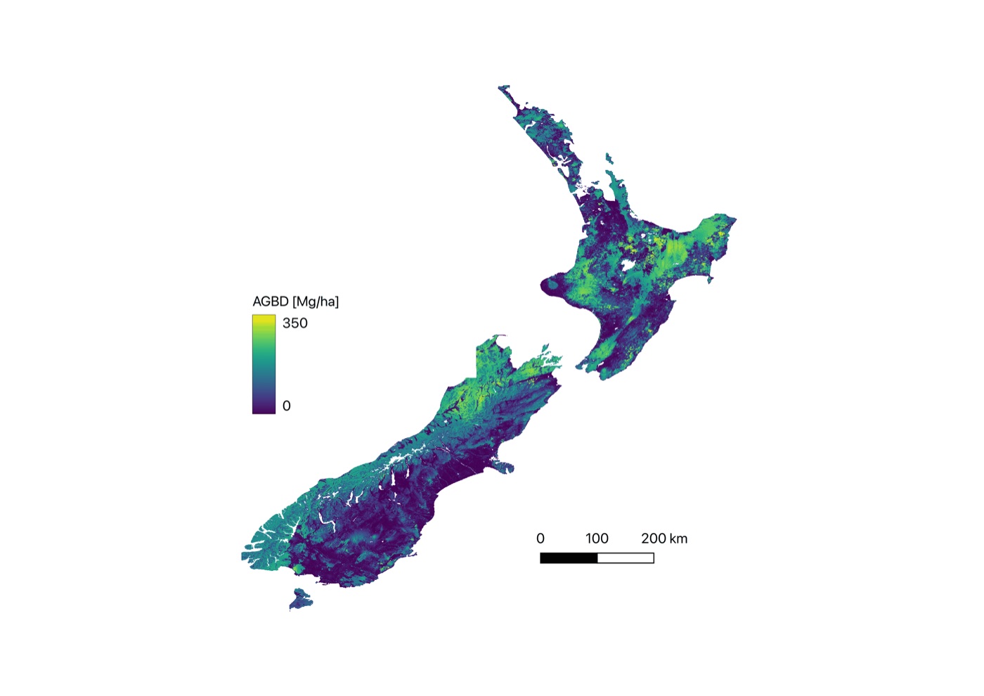
We generate calibrated AGB maps for 2020 over all 11 AGBD regions, from yearly Sentinel-2 composites, about 3 million km² in total. The maps follow ecological gradients, such as the forest belts of the Sierra Nevada and the Himalayan foothills, or the transition from the Qinling Mountains to the Wei River plains in Shaanxi, and they keep anthropogenic structure: plantations, agricultural mosaics and deforestation edges appear as sharp discontinuities. In Ghana, protected forest reserves stand out sharply from the surrounding cultivated land.
Figure 2. Calibrated AGB map of Ghana (Mg/ha), with a zoomed-in detail.


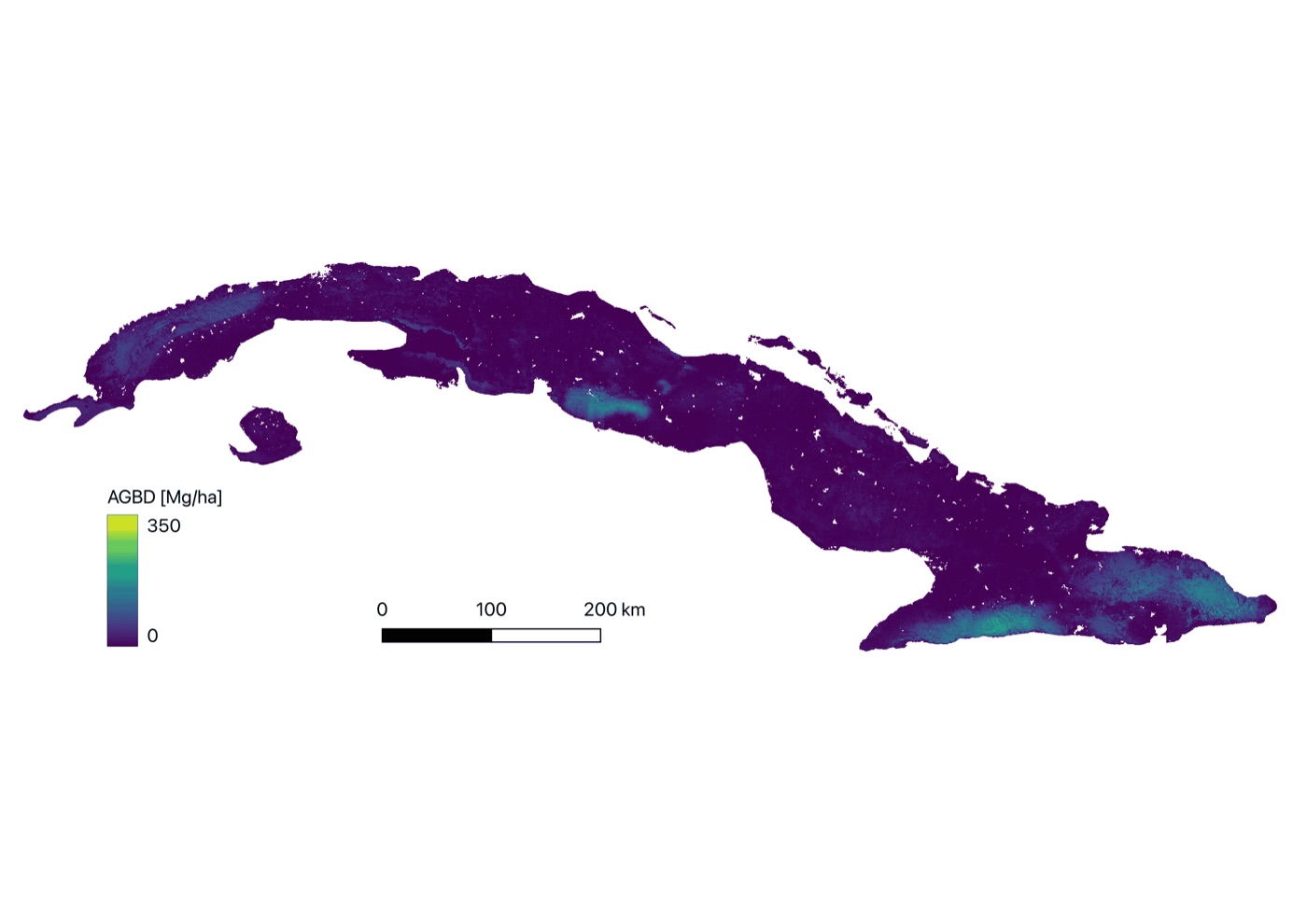
Figure 3. Calibrated dense AGB maps over the 11 regions of the AGBD dataset.
Global error measures are dominated by the many low-biomass samples. To capture the effect of calibration across the whole range, we split AGB into ten 50 Mg/ha bins and count the bins whose median bias the calibration reduces: $$\Delta B = \sum_{b=1}^{10} \mathbf{1}\big[\,|\rho^b_{post}| < |\rho^b_{map}|\,\big],$$ where $\rho^b$ is the median residual in bin $b$. Only configurations with $\Delta B = 10$ reduce bias across the full range. Removing out-of-distribution samples before fitting matters most for reaching $\Delta B = 10$; interpolating residuals rather than absolute AGB fixes the difficult 150–200 Mg/ha bin; and each added group of auxiliary variables lowers the RMSE further. The calibration still helps with only 5K footprints per tile.
| $N$ | $\nu$ | ood | pred | aux | $\lambda_{xy}$ | $\Delta B$ (↑) | MAE (↓) | RMSE (↓) | ME | |
|---|---|---|---|---|---|---|---|---|---|---|
| I | 25K | 3/2 | × | agb | base | 1000 | 7 | 29.58 | 56.76 | 0.05 |
| II | 25K | 1/2 | × | agb | base | 1000 | 7 | 28.22 | 54.47 | 0.12 |
| III | 25K | 1/2 | ✓ | agb | base | 1000 | 9 | 30.28 | 56.35 | 5.61 |
| IV | 25K | 1/2 | ✓ | agb | base | Δ | 9 | 32.30 | 59.83 | 6.25 |
| V | 25K | 1/2 | ✓ | res | base | Δ | 10 | 32.71 | 60.52 | 6.29 |
| VI | 25K | 1/2 | ✓ | res | base+local9 | Δ | 10 | 31.67 | 58.18 | 6.20 |
| VII | 25K | 1/2 | ✓ | res | base+local25 | Δ | 10 | 31.45 | 57.78 | 6.15 |
| VIII | 25K | 1/2 | ✓ | res | all9 | Δ | 10 | 31.37 | 57.62 | 6.13 |
| IX | 25K | 1/2 | ✓ | res | all25 | Δ | 10 | 31.15 | 57.22 | 6.11 |
| IX | 10K | 1/2 | ✓ | res | all25 | Δ | 10 | 31.46 | 57.47 | 6.12 |
| IX | 5K | 1/2 | ✓ | res | all25 | Δ | 10 | 31.70 | 57.67 | 6.20 |
| BioFiLM, before calibration | N/A | 57.58 | 79.91 | 32.61 | ||||||
Table 2. Kriging configurations on the per-tile held-out GEDI footprints (Mg/ha). $N$: maximum number of training footprints per tile; $\nu$: Matérn smoothness; ood: removal of out-of-distribution samples; pred: interpolate absolute AGB or residuals; aux: auxiliary variables (base; +localN: neighbourhood statistics over $N\times N$ pixels; allN: also texture); $\lambda_{xy}$: fixed or per-tile ($\Delta$) length-scale. Shaded rows (I–IV) do not reach $\Delta B = 10$ and are shown for reference; bold marks the best valid configuration. These held-out footprints differ from the AGBD test set, so errors are not comparable with Table 1.
Figure 4. Residuals ($AGB_{pred} - AGB_{GEDI}$, Mg/ha) per AGB bin on the held-out footprints, before (blue) and after (red) calibration with configuration IX. Calibration removes the over-estimation of low biomass, shifts high-biomass estimates up towards the reference, and narrows the spread of errors.
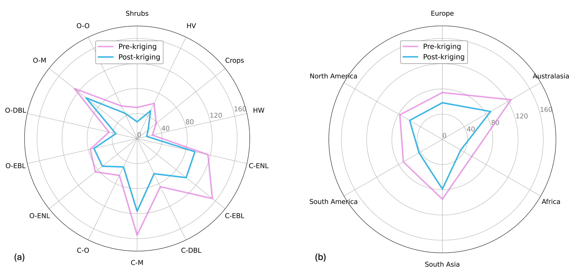
Figure 5. RMSE (Mg/ha) before (pink) and after (blue) calibration, (a) per biome and (b) per region. C-/O-: closed/open forest; ENL, EBL, DBL: evergreen needle-leaf, evergreen broad-leaf, deciduous broad-leaf; M: mixed; O: other; HV: herbaceous vegetation; HW: herbaceous wetland. The error drops in every biome and region.
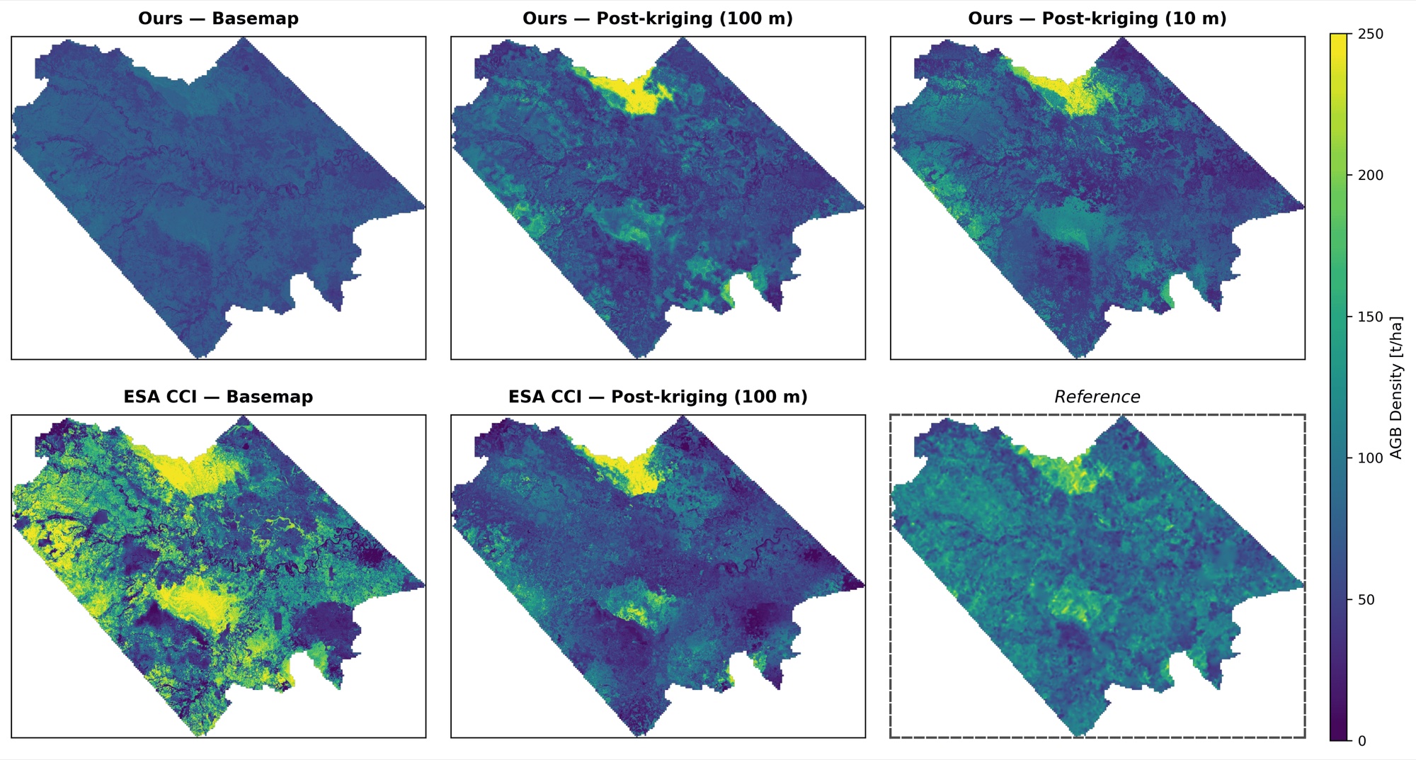
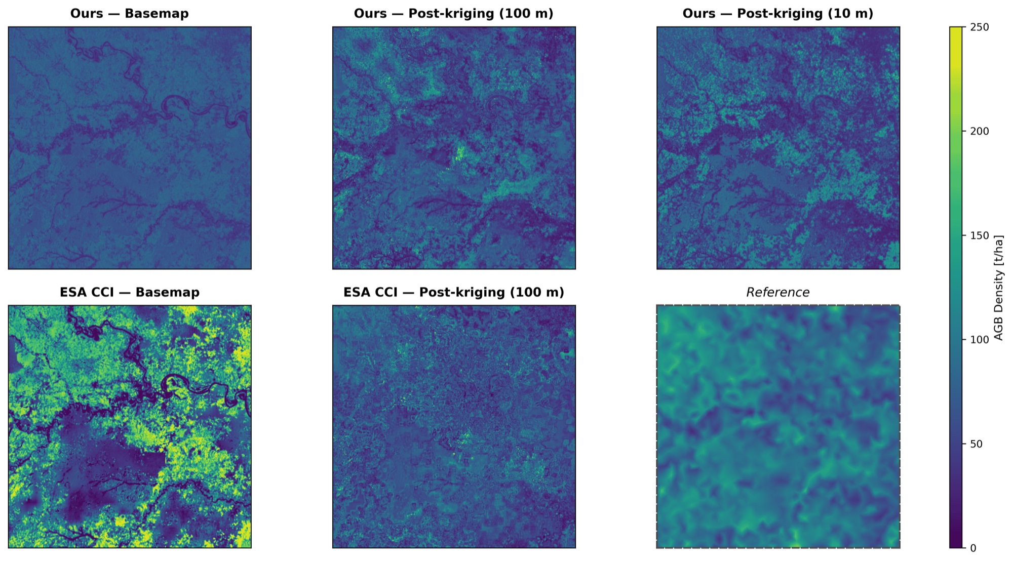
To test against independent reference data, we turn to Jambi province in Sumatra, Indonesia. No part of Southeast Asia is in AGBD, so our model never saw this region during training. The reference is a 100 m AGB map built from 80 field plots and airborne LiDAR (May et al., 2024). We calibrate both our map and the ESA CCI v6 product with GEDI L4A footprints from the same period (May 2021 – April 2022) and compare everything at 100 m.
Our map agrees much better with the reference than ESA CCI, before and after calibration. Kriging greatly improves the CCI map (RMSE −30%) and lowers our map's bias, with a small RMSE gain; the moderate agreement between GEDI and the reference data here caps what GEDI-based calibration can achieve. At a matched 100 m grid, our calibrated map still keeps finer spatial structure than CCI.
| Map | Kriging | Grid | RMSE (↓) | MAE (↓) | ME |
|---|---|---|---|---|---|
| BioFiLM (ours) | × | — | 38.31 | 30.98 | −29.43 |
| ✓ | 10 m | 38.18 | 31.64 | −22.60 | |
| ✓ | 100 m | 40.49 | 33.14 | −24.19 | |
| ESA CCI v6 | × | — | 67.58 | 55.16 | 23.17 |
| ✓ | 100 m | 47.24 | 38.48 | −24.49 |
Table 3. Errors (Mg/ha) against the Sumatra reference map, evaluated at 100 m, before and after kriging. Grid: resolution at which kriging is performed. ME: mean error (predicted − reference). Best in bold, second best underlined (by absolute value for ME).
Figure 6. AGB over the study area (t/ha), shown at 100 m. Top: our map before calibration, and after kriging at 100 m and 10 m. Bottom: ESA CCI before and after kriging, and the reference map.
Figure 7. Zoomed-in 500×500 m subset of the maps in Figure 6, at a common 100 m resolution: our calibrated map keeps more spatial detail than the CCI product.
The AGBD-GPR repository contains the BioFiLM model and
training scripts (src/model), dense map generation (src/inference, src/data_prep), the
per-tile GPR calibration (src/kriging), and the Sumatra experiments (src/sumatra). A notebook runs the
whole pipeline (compositing → inference → kriging) on a single Sentinel-2 tile, and the Sumatra analysis notebook
runs from a fresh clone with its bundled data.
git clone https://github.com/ghjuliasialelli/AGBD-GPR.git
cd AGBD-GPR
uv sync --extra notebook # pinned environment: PyTorch, GPyTorch, rasterio, ...
export AGBD_ENV=local # picks configs/local.yaml; see DATA.md for the inputs
uv run jupyter lab # example/single_tile_pipeline.ipynb
The calibrated maps can be explored in Google Earth Engine. The post-calibration AGB and standard-deviation layers, as well as the pre-calibration BioFiLM AGB and ensemble standard deviation, are released as Cloud-Optimized GeoTIFFs on the ETH Research Collection. The training data is the AGBD dataset.
Calibrating each tile independently keeps the GP tractable but can leave tiling artifacts in very homogeneous, cloudy regions such as French Guiana, and the GP uncertainty is not on a common scale across tiles. The calibration also needs GEDI footprints, so it does not apply north of 51.6°, and it inherits the known weaknesses of GEDI L4A, such as under-estimation on steep slopes and in complex forests. Promising next steps are calibrating against other reference data (e.g. ESA Biomass, NISAR) and merging the two stages into a single end-to-end model.
@unpublished{sialelli2026gpr,
author = {Sialelli, Ghjulia and Peters, Torben and Scheibenreif, Linus and Wegner, Jan Dirk and Schindler, Konrad},
title = {Gaussian Process Regression for the Calibration of Satellite-based Above-ground Biomass Estimates},
note = {Manuscript under review},
year = {2026}
}